We are releasing a database of descriptions of every neuron inside Llama-3.1-8B-Instruct, and weights of an explainer model finetuned to produce them. These descriptions have similar quality to a human expert on automated metrics, and can be generated inexpensively using an 8B-parameter model. These high-quality descriptions allow us to query and steer representations in natural languge, enabling applications such as our observability interface.
Introduction
When understanding AI systems, we often want to trace behaviors back to internal representations. This can help to uncover learned spurious correlations that degrade accuracy or fairness, surface hidden knowledge, and pinpoint the source of known issues. Once we understand these issues in terms of the representations, we can hope to fix them by intervening on or disabling the components that are responsible [1, 2, 3].
Currently, understanding representations typically requires significant human labor [4, 5, 6, 7, 8], which makes the research costly to scale and often restricts its scope to narrow sets of behaviors. Recently, automated interpretability has used AI systems to automate model understanding [2, 9, 10, 3], for example by producing human-readable descriptions of model components. Unfortunately, the resulting descriptions are often low-precision [11], and methods to increase their quality are often costly, such as expensive multi-turn interactions with explainer systems. We need cost-efficient methods for producing high-quality descriptions that scale to today's frontier systems.
To address this, we focus on the task of neuron description, which is a subcomponent of many interpretability procedures. We introduce a method for automatically producing high-quality descriptions of neurons inside language models. Our approach adapts recent work [9, 3] where an explainer model is provided data about a subject model, prompted to make hypotheses that explain the data, and hypotheses are evaluated using an automated scoring procedure. Our main contributions are:
- sampling a diverse pool of descriptions and selecting the best one using a fine-tuned scorer as a proxy for human judgment
- using distillation to transfer successful description patterns to a new model
These improvements allow for high-quality descriptions with a computational cost of approximately $0.046 per neuron (see Appendix for the cost breakdown).
We apply this procedure to produce a database of descriptions of all 458,752 MLP neurons inside Llama-3.1-8B-Instruct. To benchmark their quality, we manually annotated a subset of neurons by hand (see above for examples). The automated descriptions are qualitatively similar to human descriptions and score slightly better on our automated quality metrics (average score of vs. ). We are planning to release both the description generator and scorer models as well as the dataset of neuron descriptions.
Our resulting database supports investigation of arbitrary model behaviors by revealing human-interpretable descriptions of internal features influencing those behaviors. We exploit this in our observability interface (described in a parallel write-up), which allows users to understand behaviors in terms of the neuron representations, then automatically steer model behavior by editing families of neurons, for instance those associated with a given spurious cue. Natural language descriptions of neurons are key to this, as they enable semantic retrieval, clustering, and editing of neurons in terms of human-understandable concepts.
Automated Description of Neuron Behavior
Problem Statement and Approach
Given a transformer model or other deep neural network, a feature is any function from its representation to the real numbers. We will focus on neuron features—the activation value of a specific neuron—but our methods apply to arbitrary features, such as those produced by sparse auto-encoders (SAEs) [12, 13], and even nonlinear features [14]. See Discussion for why we chose to describe neurons instead of SAE features.
Formally, we consider a subject model whose representations we want to investigate, and assume that this model takes inputs from a domain . For a feature , our goal is to produce a natural language description that accurately predicts the behavior of . We will formalize this later through a simulator model , which predicts an activation value given an input and description . Finally, our goal is to train an explainer model that produces natural language descriptions for a given feature .
We build on Bills et al. [9], which used prompted versions of GPT-4 as both the simulator and explainer models to describe neurons in GPT-2. We fine-tune both the simulator and explainer models and augment quality using best-of- sampling, which together improve performance while keeping cost low.
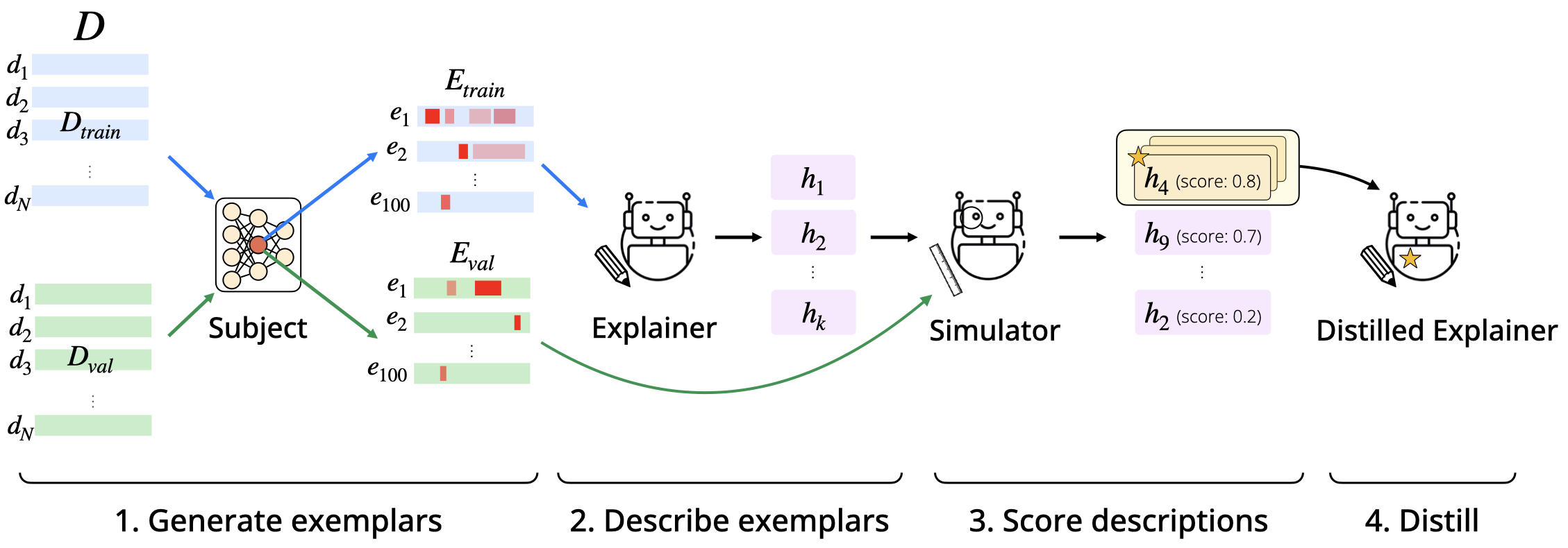
In more detail, our method depicted above has several steps:
- Generate exemplars: we construct a large corpus of diverse inputs to the model, and use inputs where is largest as an exemplar-based summary of .
- Describe exemplars: we either prompt or train a language model to produce a description of based on the exemplars.
- Score descriptions: We score descriptions by how well they predict the behavior of on held-out inputs. We do this using a simulator that predicts an activation value and compute the average correlation of with across the held-out set. We score all descriptions and rank them based on their scores.
- Distill: finally, we distill a new model using the top-scoring descriptions.
The final distilled model is only 8B parameters and outperforms GPT-4o-mini at generating descriptions.
Generating exemplars
We summarize a feature's behavior using its activation pattern over text excerpts [9]. Given a dataset of text excerpts, we take the excerpts on which takes the largest values, and call the resulting sets of exemplars . More precisely, for an input of length , yields an activation vector of length corresponding to 's value on each prefix of . The max-activating exemplars are the inputs for which the maximum over these values is largest.
In our experiments, we describe neuron features in Llama-3.1-8B-Instruct. This model uses gated MLPs, which can take on both
positive and negative activation values. Specifically, the activation of neuron is calculated as the product of a SiLU-transformed linear function times a second linear function [15]:
where is the pre-MLP value of the residual stream. Since activations can be both positive and negative, we construct separate exemplar sets and for the most-positive and most-negative exemplars for each feature. The activation patterns for positive and negative polarities are often related, and we found several neurons that had interesting relationships between the two polarities, which we highlight below.
For the dataset , since our subject model is a chat model pre-trained on web text, we combine both chat and web data to surface a wide range of possible neuron behaviors. Specifically, we take to be the entire LMSYS-Chat-1M dataset [16] together with a 10B token subset of Fineweb [17]. We sample chat interactions of length 95 tokens1We take the first 95 token IDs and include conversations that are less than 95 tokens from LMSYS-Chat, including the 30 token Llama chat prefix. Text sequences from Fineweb are randomly sampled to have a length of 65 contiguous tokens, where each sequence is sampled from a single document. We prepend Fineweb sequences with the 30 token Llama chat prefix (reproduced below) so that they also have length 95 (effectively treating each Fineweb sequence as a user message to the chat model).
We subdivide into training (), validation (), and test () splits of equal size that contain equal numbers of Fineweb and LMSYS sequences. We will later use and as held-out data to measure the quality of our descriptions.
In principle, we could consider exemplars spanning a wider range of the activation distribution of each feature, rather than only looking at the top values. We used top-activating exemplars since past work has shown that they often yield useful insights [18, 19, 2, 3, 20]. However, we sometimes observe cases where model behaviors we seek to understand depend on neuron activity in lower quantiles.2For example, highly attributed neurons have activations that are outside of this top percentile, and our descriptions might not describe those kinds of sequences. We plan to expand descriptions to capture these lower quantiles in future work.
Describing exemplars
After computing exemplars over for each feature, we use a language model (the explainer) to generate a set of candidate hypotheses that explain and . These hypotheses are expressed in open-ended natural lanugage, following prior work [2, 9, 3]. More sophisticated hypotheses could also be implemented as programs or structured causal models that approximate the behavior of the subject model on inputs of interest.
To obtain hypotheses, we prompt the explainer model with instructions, few-shot examples, and data (exemplars) to explain.
Description quality varies substantially with the contents of this prompt and the format in which data is presented to the explainer. Prior work [9] represented each exemplar as a list of tab-separated (token, activation) pairs.3Activations are normalized between 0 and 10. We found that this paired format is difficult for the explainer to ingest, and instead replace per-token
activation values with inline delimiters ({{}}) to highlight activations above a certain quantile, similarly to [21].4To ensure we provide useful signal to the explainer about each sequence, quantiles are determined dynamically so that a minimum of three highlighted tokens per prompt are shown to the explainer.
Few-shot examples. We provide the explainer with few-shot examples of exemplars and descriptions drawn from the neuron puzzles in [9] with known ground-truth descriptions. We find that a single example improves description quality more than additional examples (see Figure 7), so for every prompt, we sample one few-shot example from the 19 neuron puzzles and provide it to the explainer along with the neuron data to explain. We provide an example prompt in full below.
Best-of- sampling. Our most effective strategy for improving description quality involves increasing the number and diversity of hypotheses produced by the explainer, so that we can then select the hypothesis that best explains the data. For each feature, we sample hypotheses from the explainer model. We vary the prompt across samples to further increase diversity, by:
- varying the number of exemplars (10-20) included in the prompt, sampled from
- sampling the few-shot example from a pool of few-shot examples
This strategy produces a pool of candidate hypotheses for explaining . As an example, see the 5 hypotheses produced for the positive activations of neuron L31/N8883 below:
Scoring descriptions
Given a pool of candidate hypotheses, we wish to rank them based on how well they explain the data. We do so using a set of held-out exemplars computed from . For , we take the union of the top highest-activating exemplars across , together with randomly sampled sequences from , following [9].5We include random text sequences to penalize broad descriptions: given a precise description, the simulator should accurately predict high activation on top-activating sequences, and low activation on random sequences. We score each hypothesis based on how well it predicts activation values across .
To compute a numerical score, we need a simulator model that predicts activations on given a hypothesis . Given , we obtain a simulation score by computing and across all prefixes of all exemplars in , aggregating these into a single set, and computing the Pearson correlation coefficient .
In past work [9, 22], the simulator is a language model prompted to use the hypothesis to predict the feature's per-token normalized and discretized activation level. The simulated activation is simply the the numbers 0-10 weighted by the probability of the tokens '0', ..., '10'.6The requirement of access to logprobs means we are unable to use most proprietary models as simluators. In particular, Bills et al. design a prompt called "all at once" to get simulated activations in a single forward pass instead of doing a forward pass per simulated token. However, even with this trick we found simulation to be too slow for two reasons: (i) the language model must be powerful (and therefore, big) enough to be able to do the task with just prompting, and (ii) the prompt is long due to the extra tokens that are required in the prompt (tab separator and placeholder tokens from Bills et al.). This made it expensive for us to simulate hypotheses per feature for all neurons in the subject model.
Fine-tuning a simulator. To produce a small, fast, and accurate simulator, we fine-tune Llama-3.1-8B-Instruct to directly predict per-token activations given and . Fine-tuning allows us to use smaller models, and the task of directly predicting the output (integer from 0-10) gets rid of the extra tokens, making the prompt much shorter.
An ideal simulator would faithfully predict activations on given an accurate description of the neuron. To avoid distribution shift, our training dataset would thus ideally contain accurate feature descriptions,
which are expensive to obtain by hand. We therefore use a two-stage process: first, we fine-tune Llama-3.1-8B-Instruct using randomly sampled (unranked) hypotheses from the hypotheses generated by the explainer for each neuron, then we fine-tune a second simulator using the best of descriptions for each neuron as selected using the first-stage simulator.
Training datasets. We train the first-stage and final simulators to directly predict ground-truth neuron activation values normalized and discretized to be in the range .
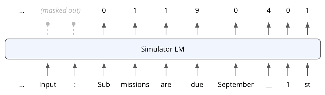
An example training datapoint is shown below for = "phrases indicating due dates or deadlines for submissions or applications" and = [' Sub', 'missions', ' are', ' due', ' September', ' ', '1', 'st']. The input is a description of the neuron followed by the input exemplar:
And the training objective is to predict the normalized and discretized ground-truth activation at each token position of , instead of predicting the next token in the exemplar sequence:7We mask out all other tokens positions when computing the loss.
Our training data for fine-tuning the simulator does not include a system prompt or few-shot examples, which makes a forward pass more efficient compared to a non fine-tuned prompt-based simulator.
To construct the training data, we randomly sample 2000 neurons across all layers, and additionally include all neurons with at least one description that mentions at least one special token (109 neurons).
This results in exemplar sets ( and for each neuron). We pair each exemplar with a randomly sampled hypothesis among the hypotheses generated by the explainer for that feature. This leads in total to input sequences, and we fine-tune the first-stage simulator on this dataset with batch size 64 for 1500 steps.
We next sample a new dataset of 2000 neurons and compute simulation scores using the first-stage simulator to rank the hypotheses produced by the explainer. To train the second simulator, we sample 5 exemplars out of the exemplars in , and pair them with the best-scoring hypothesis (out of the pool of ) for that feature. We fine-tune the second-stage simulator on the resulting dataset with batch size 32 for 650 steps. We subsequently use this simulator to select best of descriptions for creating our descriptions dataset and fine-tuning an automated explainer model. Code for training the simulator model will be available in our code repository.
Special tokens. Since the simulator uses the same tokenizer as the subject model, the simulator was initially unable to score descriptions containing special tokens (e.g. “this neuron activates strongly on <|begin_of_text|>”). To solve this problem, we added 4 new tokens to the tokenizer's vocabulary, and mapped all instances of special tokens in the input to the new tokens:
<|begin_of_text|>↦<||begin_of_text||><|start_header_id|>↦<||start_header_id||><|end-header_id|>↦<||end-header_id||><|eot_id|>↦<||eot_id||>
Distilling an automated explainer model
We further fine-tune an explainer model on the best-of- descriptions to distill a cheap and high-quality explainer. We do this for
two models, the proprietary GPT-4o-mini and open-weight Llama-3.1-8B-Instruct.
Distilling GPT-4o-mini. To produce descriptions to train on, we generate hypotheses per neuron using GPT-4o-mini as a base explainer (as described in Description generation), then take the highest-scoring hypothesis according to the simulation score from Scoring descriptions).
We compute these descriptions for randomly-selected neurons (both positive and negative polarity). We then fine-tune an explainer to predict this top description given a set of 10-20 top-activating exemplars from , using the same format as in Description generation, but without few-shot examples. We fine-tune GPT-4o-mini on this dataset for 1 epoch to obtain a distilled explainer model.
To produce the descriptions in our database, we further run best-of- with this new explainer for . We sampled 10-20 top-activating exemplars per neuron from , and did not provide the fine-tuned explainer with few-shot examples.
Distilling Llama-3.1-8B-Instruct. We further distilled the fine-tuned GPT-4o-mini model to a Llama-3.1-8B-Instruct model.
We used descriptions of 8000 neurons randomly sampled from our database to fine-tune the model (recall these are best-of-25 samples
from the distilled GPT-4o-mini explainer). We use the same input format with 10-20 top-activating exemplars as before.
This fine-tuned explainer based on Llama-3.1-8B-Instruct outperforms finetuned GPT-4o-mini as measured by our simulation score
(see Figure 5).8This explainer is bottlenecked by GPUs, while the GPT-4o-mini explainer is bottlenecked by API calls. We were able to obtain descriptions more efficiently using the GPT-4o-mini explainer, and are releasing those descriptions in our description database.
The weights of the fine-tuned explainer will be available in our code respository.
Results
We next study the descriptions we generate, evaluating their quality and comparing to human-generated descriptions and baselines. We label every MLP neuron in Llama-3.1-8B-Instruct using best-of-25 from the distilled GPT-4o-mini model, as described in
Distilling an automated explainer model.
We also label subsets of these MLP neurons with other methods to allow for quantitative comparisons.
Llama-3.1-8B-Instruct contains a total of 458,752 MLP neurons (14,336 per layer across 32 layers), and we label both the positive and negative
direction for each neuron.
In the sections below, we first visualize the overall distribution of simulation scores across layers, then compare to human descriptions and find that our automated descriptions score higher. We then examine an interesting phenomenon: the best-of- description score is a nearly-perfect power law function of , enabling us to predict performance as a function of computation. Finally, we run several ablations and find that our simulation scores are significantly higher than baseline methods.
With the exception of the comparison against human descriptions (which used ), all scores reported in this section were computed using due to the cost of evaluating on .9It would take 116 GPU hours to evaluate the best description for all neurons in Llama-3.1-8B-Instruct. Therefore, our emphasis in the following sections is not on the absolute scores we achieve but rather the comparisons we make against previous work and baselines. (An analysis of 100 random neurons shows that scores on are highly correlated with performance on and differ by only 0.04 on average; see Figure 10.)
Description scores by layer
We visualize the distribution of scores achieved by the best descriptions sampled using the distilled GPT-4o-mini explainer, scored using the fine-tuned simulator. In Figure 1, we see that the average score decreases from layer 1 to layer 11, but increases again after that. In Figure 9, we show that this trend is present for the non-distilled GPT-4o-mini explainer, and the distilled Llama-3.1-8B-Instruct explainer as well.
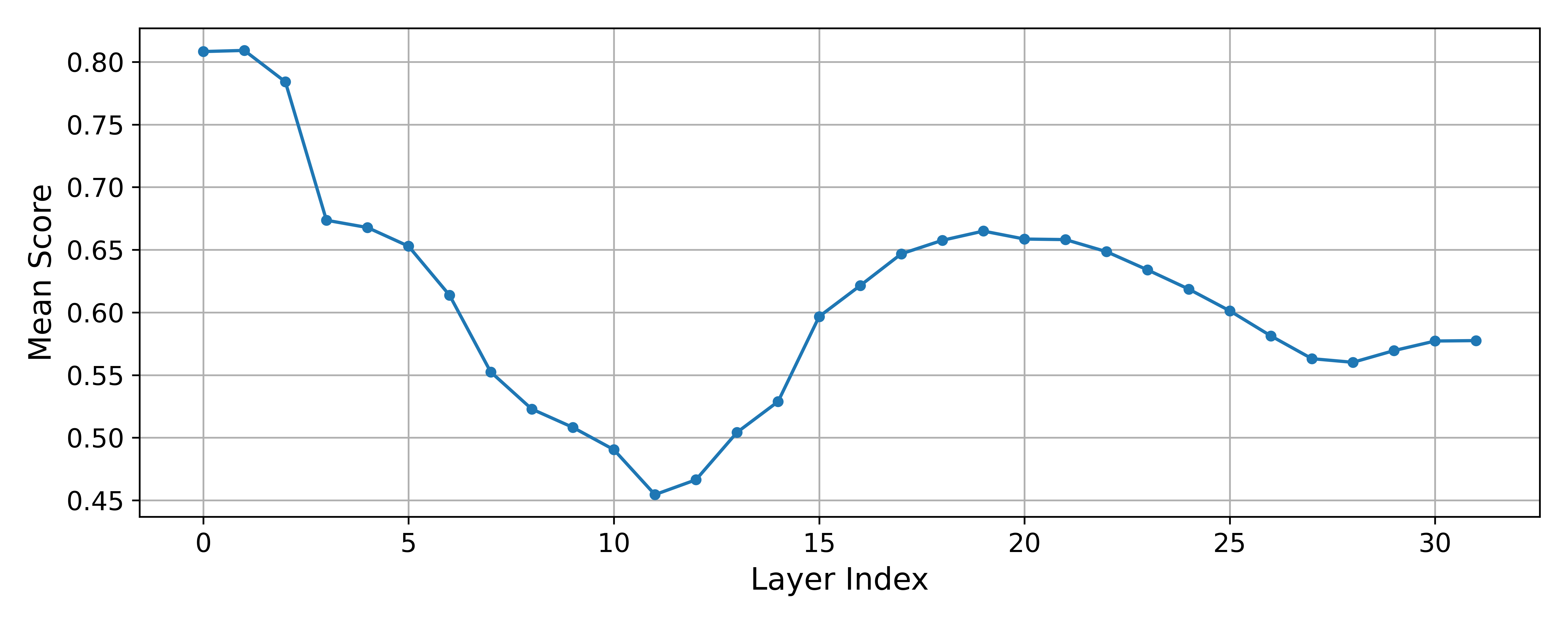
Figure 1: The average score per layer does not follow a strict monotonic trend. Scores are from the best-of-25 descriptions from the distilled GPT-4o-mini explainer, averaged over all neurons and both polarities per layer.
Following Bills et al. we visualize the distribution of scores for each layer in Figure 2. We found that our per-layer distributions look different from the Bills et al.'s—our distributions have modes close to or above 0.5, while Bills et al.'s modes are mostly close to 0. Interestingly, for some layers our distributions are bimodal (see layer 14-18 and 30-31).
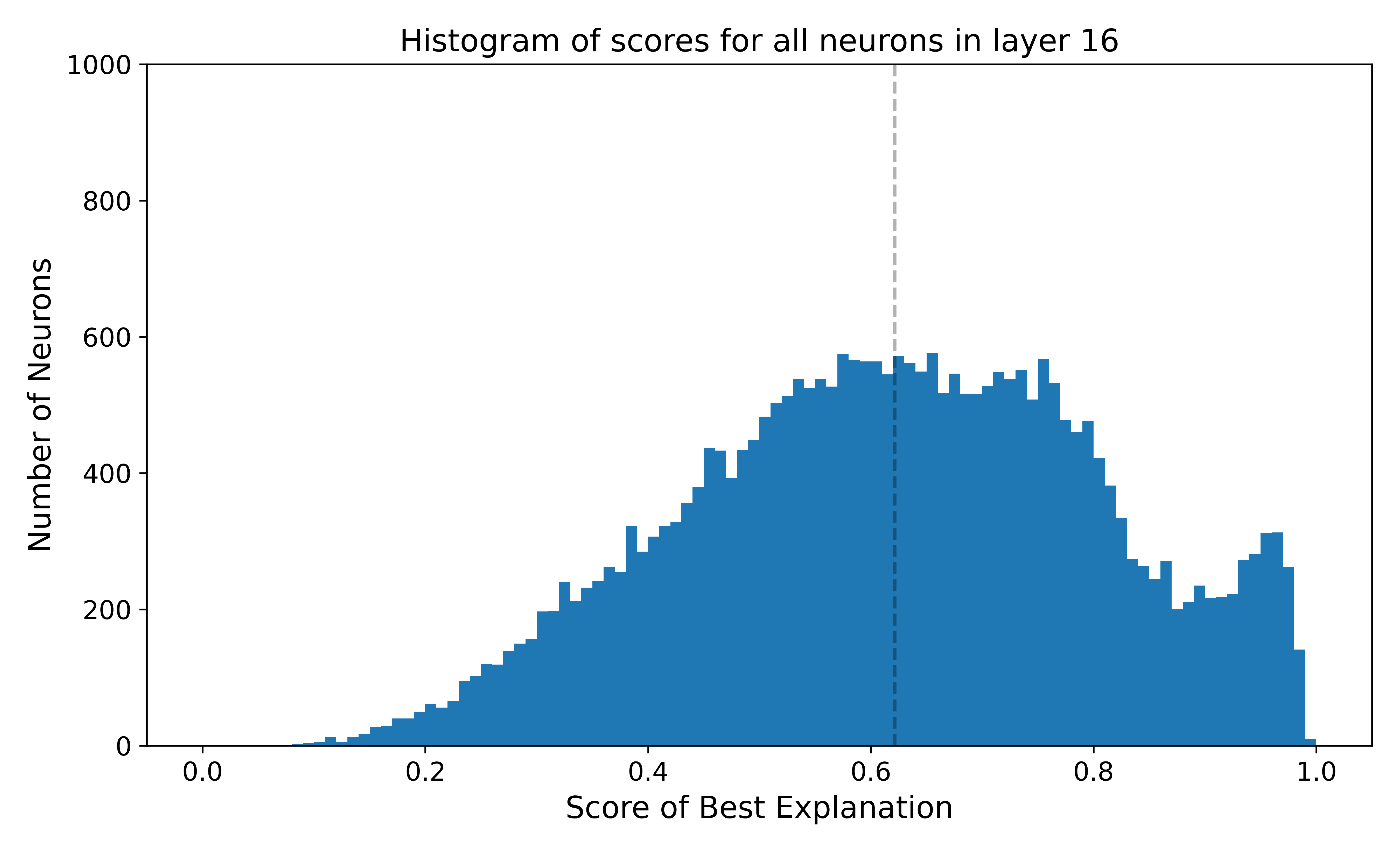
Figure 2: Our scores are much higher than those shown in Bills et al. Notably, some layers (14-18 and 30-31) have a bimodal distribtion of scores. The histograms were constructed using scores achieved by the best-of-25 descriptions from the distilled GPT-4o-mini explainer per layer. The dotted vertical line corresponds to the mean.
Descriptions out-perform human descriptions
We compare descriptions produced by our fine-tuned explainer to descriptions written by a human expert, and find that automated descriptions consistently outperform human descriptions, while following the same neuron-level trends.
Human description generation. To construct the dataset of human descriptions, four human experts wrote descriptions for several randomly sampled neurons, and the human annotator with consistently higher scores (who was one of the authors) was selected to manually construct a larger dataset. For 100 randomly sampled neurons from across all layers of the subject model, the expert annotator was given the same set of exemplars () as the explainer (for either the positive or negative polarity, sampled at random for each neuron), and instructed to write descriptions of the neuron's behavior.10The human annotator did not have access to the automated explainer's descriptions. The human was given access to the simulator and had the opportunity to iteratively refine their description to hill-climb on the simulator's score on . Across all neurons explained, the annotator wrote and scored an average of 3.01 descriptions per neuron. The human annotator spent 6 hours constructing the dataset, or around 3.6 minutes per neuron.
Comparison to automated descriptions. In order to make a fair comparison, for both the human and automated descriptions, we selected the top-scoring description for each neuron according to , and evaluated it on . Figure 3 gives per-neuron comparisons of description scores for human and automated descriptions across the 100 neurons. Using the fine-tuned simulator, the average score of automated descriptions is 0.61, compared to 0.55 for human descriptions, with a statistically significant difference (paired t-test with p-value=).
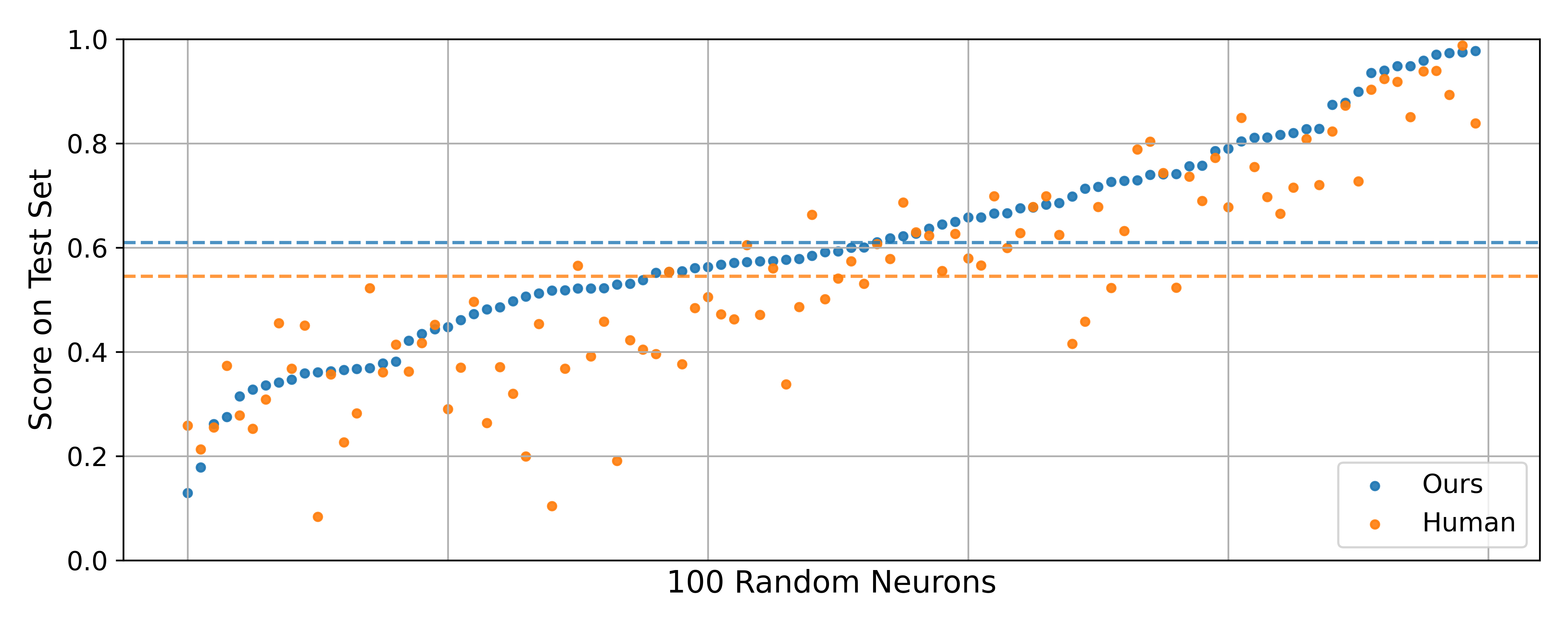
Figure 3: Our automated descriptions score higher than human expert's descriptions both on average (dotted line) and at a per-neuron level for both fine-tuned and non-finetuned simulator. Our explainer is better for 75/100 neurons for fine-tuned and 65/100 neurons for non-finetuned. Each point represents the score corresponding to the highest-scoring description of a particular polarity of a neuron. "Ours" corresponds to using the distilled GPT-4o-mini explainer to sample 25 descriptions, and "Human" corresponds to a human expert who was allowed to optimize the score (3.01 descriptions on average per neuron). The neurons are sorted by the score achieved by our explainer.
In addition to this, since our simulator was fine-tuned on descriptions produced by an automated explainer similar to the one we evaluated, we also scored the descriptions using a non-finetuned simulator—a Llama-3.1-70B-Instruct prompted using the simulation method from Bills et al.11Llama-3.1-70B-Instruct is instructed to predict a neuron's activation level normalized from 0 to 10 on each token, and the simulator output is the expected value according to the probabilities of the tokens '0' to '10'. The average simulation score according to this simulator is 0.38 for automated descriptions, and 0.34 for human descriptions (paired t-test with p-value=).
There are several additional things to note from Figure 3:
- The scores from the non-finetuned simulator are lower than the fine-tuned simulator. This is expected since fine-tuning makes the simulator better at the task of simulating than prompting, especially on in-distribution data. We also did not explore better prompting formats (system prompt and few-shot examples) for the non-finetuned simulator beyond the one used in Bills et al.
- Neuron description scores are correlated between human and automated descriptions for both simulators. This is not enough to guarantee that the simulator is aligned with human preferences, but is nonetheless a good sign that the simulator and human agree on the difficulty of the task at a per-neuron level.
Scaling description quality
It's obvious that sampling more diverse decriptions improves the quality of the best description. But how much better is it to sample 5 descriptions vs 50? We plotted the average score of the best description from doing best-of- using a non-finetuned GPT-4o-mini explainer against , and found that the relationship follows a power law, with rapid improvements coming from sampling more than one description. In Figure 4, we show that a power law fitted using predicts the average score for .
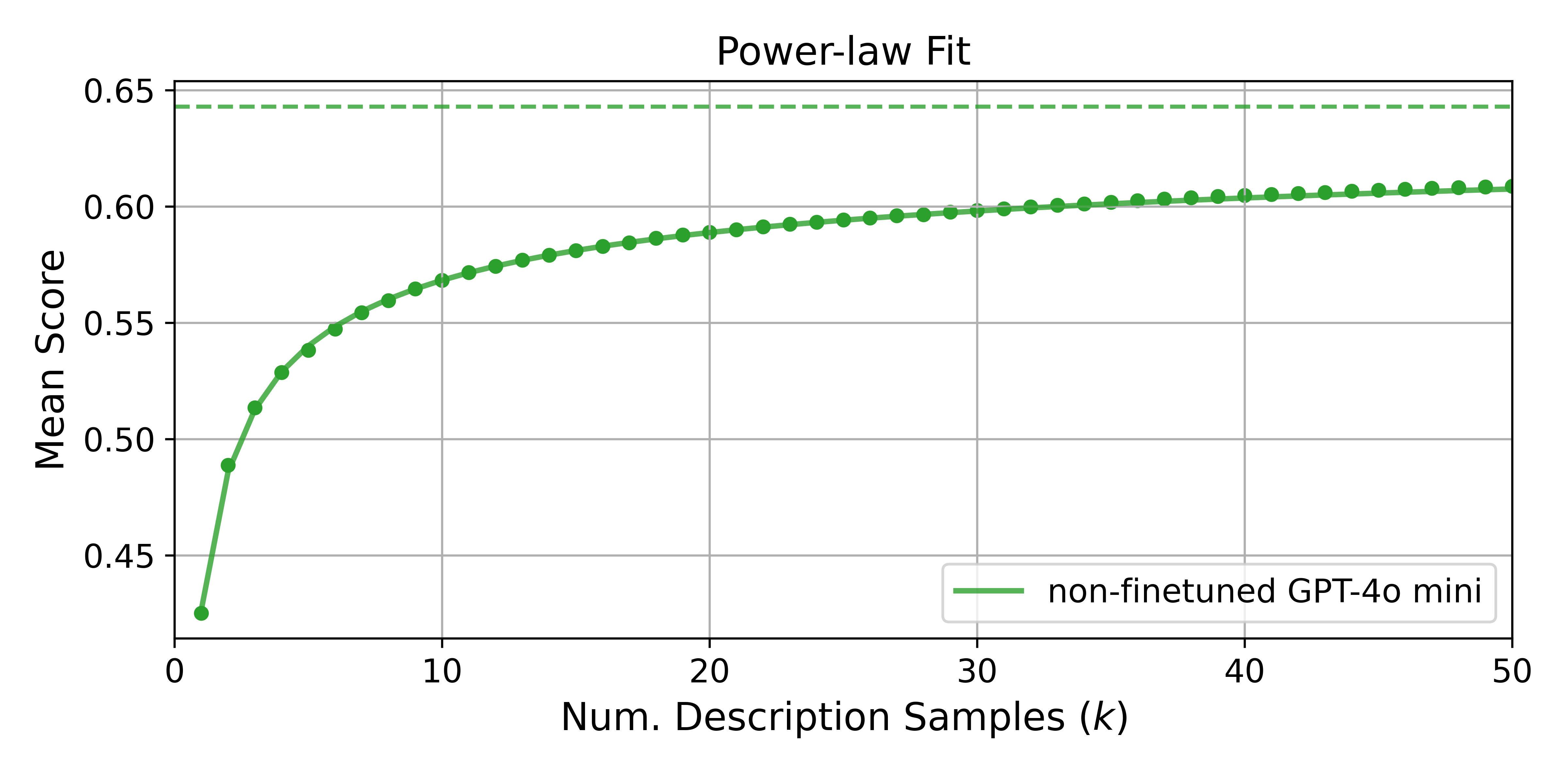
Figure 4: Average score of best-of- descriptions follows a power law as a function of . We used a non-finetuned GPT-4o-mini explainer to sample descriptions per neuron, and fitted a power law to the scores for . The dots correspond to the actual average scores, and the line corresponds to the fitted power law. The dotted line is the asymptote of the fitted power law. Scores are averaged over 2000 random neurons (both polarities) across all layers.
Doing best-of- is a simple way to improve scores, but the benefits diminish quickly. In Figure 5, we show that distilling best-of-50 descriptions from GPT-4o-mini to fine-tune GPT-4o-mini, and doing best-of- using the fine-tuned model yields higher scores with fewer samples compared to the non-finetuned model. For example, to get the same score as a distilled GPT-4o-mini explainer gets using 50 samples, we would need to sample 150 desciptions with a non-finetuned GPT-4o-mini explainer. Taking it one step further and distilling the distilled GPT-4o-mini model to Llama-3.1-8B-Instruct leads to improvements but the effect is much smaller. Fitting a power law to the distilled models shows that indeed the distilled models have higher asymptotes than their source explainers (see Figure 5).
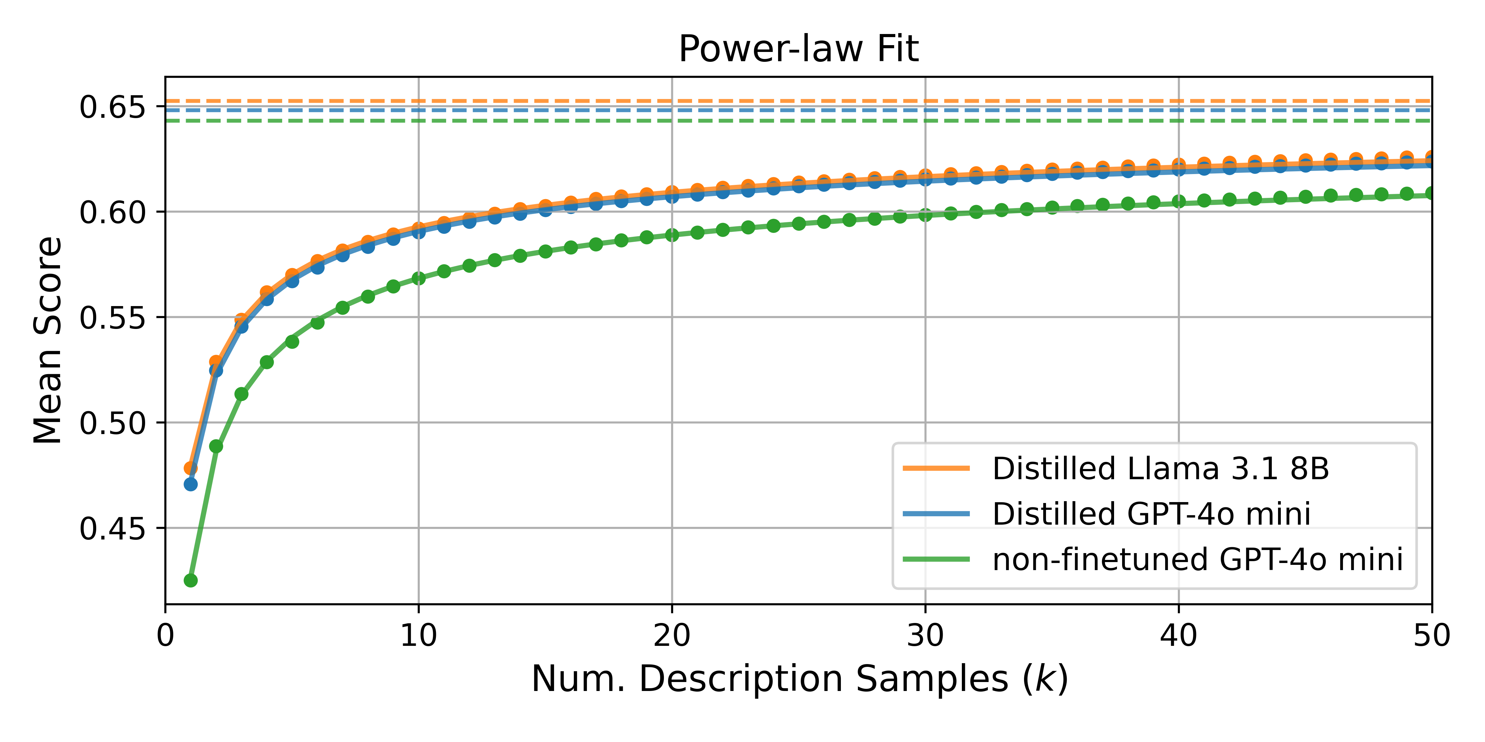
Figure 5: Distilling best-of- descriptions allows us to achieve the same description quality with less sampling compared to the data source. "Distilled GPT-4o-mini" was trained using best-of-50 descriptions from GPT-4o-mini, and "Distilled Llama 3.1 8B" was trained using best-of-25 descriptions from distilled GPT-4o-mini. For each explainer, we fitted a power law to the scores for . The dotted line is the asymptote of the fitted power law. Scores are averaged over 2000 random neurons (both polarities) across all layers, with no overlap between these neurons and the neurons used to distill the explainer models.
Ablation studies for Explainer Prompt
Prompt format. In Describing Exemplars, we hypothesized that using a (token, activation) format might be challenging for the explainer to ingest due to the text being broken up by the activation values. In Figure 6, we show that descriptions generated using the (token, activation) format achieves lower simulation scores using the fine-tuned simulator.
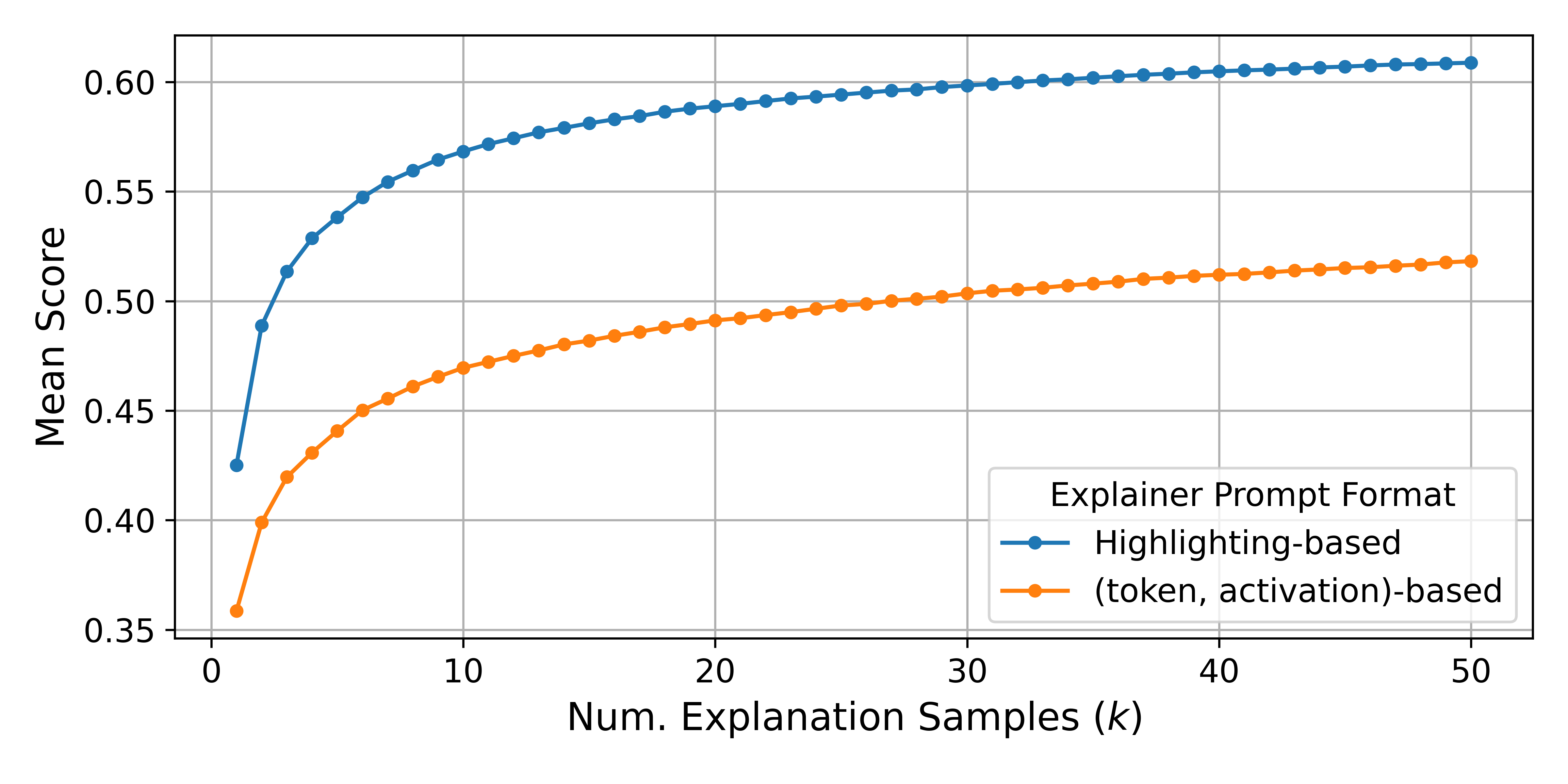
Figure 6: When constructing the prompt for the explainer, including activation values in (token, activation) format from Bills et al. results in worse simulation scores compared to our format (highlighting highly activating tokens). Scores are from a non-finetuned GPT-4o-mini explainer, averaged over 2000 random neurons for the finetuned simulator, and 100 neurons for the non-finetuned simulator. The lines connecting the dots are purely for visual clarity.
Using the finetuned simulator to compare two different prompt formats is not entirely fair since the simulator was fine-tuned on the descriptions generated using our highlighting strategy. Therefore, we also report scores for the non fine-tuned simulator (albeit with much less neurons due to the cost). Using the (token, activation) format yields worse scores in this case as well.12The scores we report for the (token, activation) format are higher than the average score reported in [9], which is 0.151. There are many differences between our setups that could contribute to this difference, including the difference in subject model and the dataset used to get the exemplars.
Number of few-shot examples. Here, we confirm that using fewer few-shot examples results in better average scores. Figure 7 shows that including more few-shot examples in the explainer prompt yields worse scores across all values of for the non-finetuned GPT-4o-mini explainer. We hypothesize that this is because descriptions are more diverse with fewer few-shot examples, although this does not explain the behavior at .
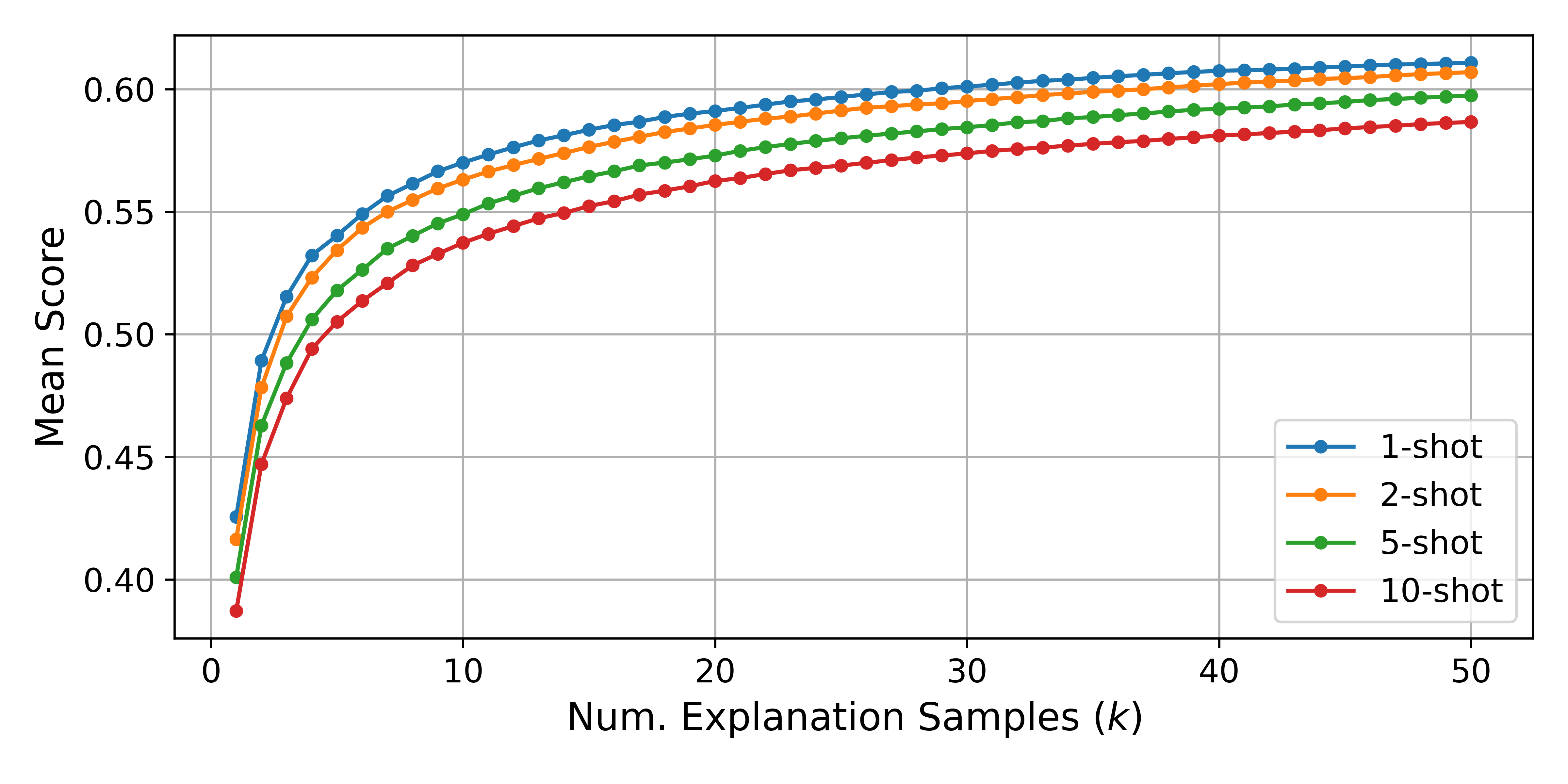
Figure 7: Using more few-shot examples in the description-generating prompt results in worse simulation scores across all values of . Scores are from a non-finetuned GPT-4o-mini explainer, averaged over 1000 random neurons. The lines connecting the dots are purely for visual clarity.
Chain-of-thought prompting. We tried adding explicit reasoning steps to the prompt to see if it would improve the quality of the descriptions. We show the exact prompt template used below (we constructed 2 few-shot examples that follow the reasoning steps outlined in the prompt).
Figure 8 shows that using chain-of-thought prompting results in worse simulation scores, which we hypothesize is due to the reduction in description diversity.
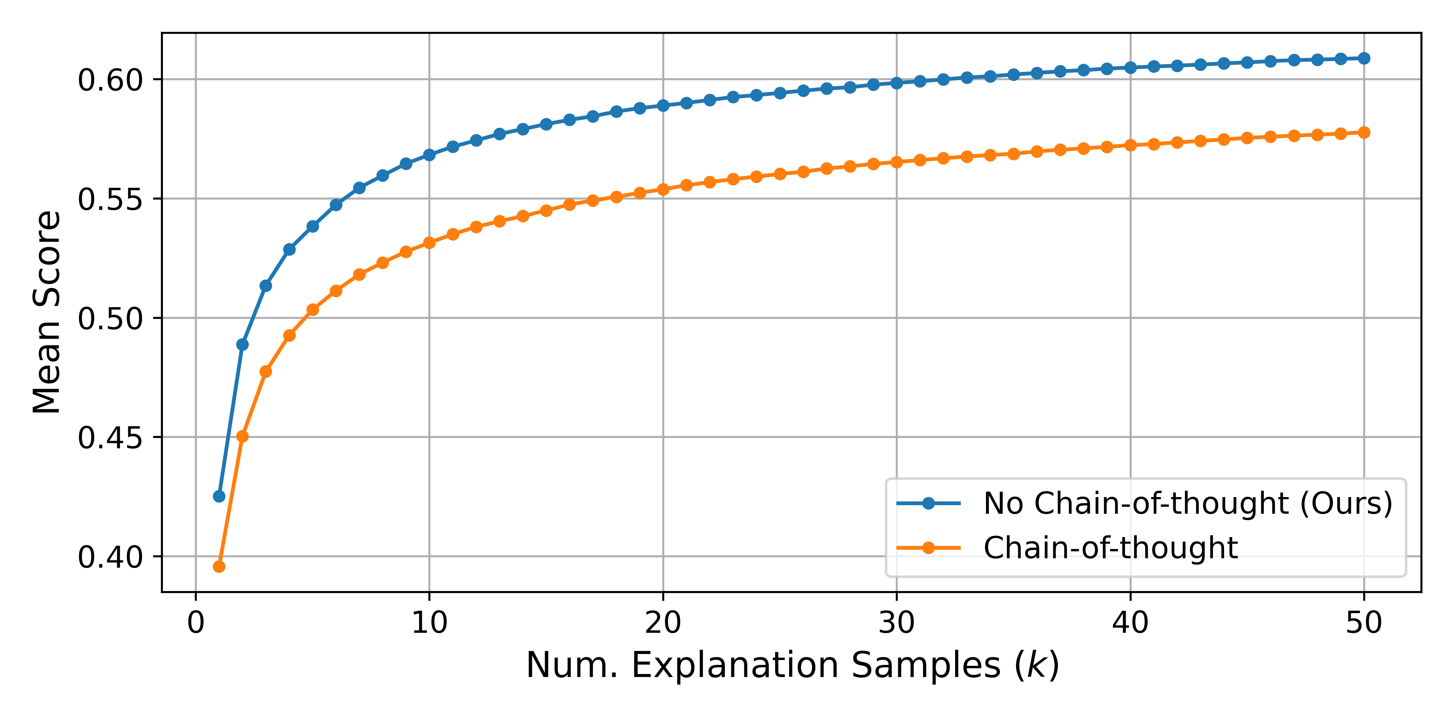
Figure 8: Using chain-of-thought prompting in the description-generating prompt results in worse scores. SScores are from a non-finetuned GPT-4o-mini explainer, averaged over 2000 random neurons. The lines connecting the dots are purely for visual clarity.
Discussion
Limitations
Potential misalignment between simulator and human understanding. Fine-tuning a simulator enables us to score all neurons inside Llama-3.1-8B-Instruct more efficiently.
But through the process of fine-tuning, the simulator can learn uninterpretable patterns between the description and neuron activations, and produce higher scores for descriptions that are less interpretable to humans. Future work could explicitly train the simulator to be aligned with human understanding by collecting activations that a human would have produced given an description.
Describing only top-activating exemplars. Our descriptions were scored on mostly top-activating exemplars which means that they are not representative of the full behavior of the neuron across all quantiles. At the same time, our pipeline can be easily modified to describe exemplars collected from lower quantiles. We leave this as future work.
Potential overfitting of best-of- descriptions to . In principle, given a large enough number of samples , the best-of- description might overfit to the patterns in , and evaluating these descriptions on might then give unrealistic scores relative to the held-out set . In practice, we observe that performance on and are similar and highly correlated for , so we do not believe this poses a major problem for our method or results, although it may bias some of our absolute scores upward by a small factor. (See Figure 10.)
Tokenization Llama models use byte-pair encoding (BPE) that break up certain characters such that decoding certain token ids might result in nonsensical tokens. This is an issue when constructing the prompt for the explainer model because highlighting scheme works at a token-level. This is also an issue for prompt-based simulators (as mentioned by Bills et al.[9]), which does not apply to us since we fine-tune the simulator.
Describing the what, not the how. Many interpretability techniques focus on what information models compute, describing individual representations and detecting when they are active in a model's computation. Like these other description procedures [2, 19, 3, 9], our expalantion pipeline does not describe how model decisions are made, or how downstream representations are produced from upstream ones. The descriptions our pipeline produces could be useful inputs to procedures that produce causal descriptions of model behavior, but do not themselves provide an algorithmic description of comuptations inside models.
Applied Interpretability
Despite these limitations, we find that the neuron descriptions produced by our pipeline already enable users of our observability interface to pinpoint previously unknown spurious correlations inside Llama-3.1-8B-Instruct that underlie known model failures. In turn, incorporation of the descriptions into the interface surfaces improvements to our pipeline that would make descriptions more useful for real-world model understanding tasks. For instance, pilot experiments using the interface have revealed:
- The importance of precise descriptions (and a precision-based scoring metric) — applications such as steering benefit from accurate prediction not only of contexts in which a feature is active, but related contexts where it is not relevant.
- The usefulness of clustering: even human-interpretable descriptions of model components still represent large sources of data that require additional parsing before they are useful to humans. The AI linter system in our current interface clusters neurons relevant to user queries, but sometimes fails to surface informative clusters. Interactive paradigms that incorporate user feedback could help guide the linter to provide clusters relevant to concepts a user wanted to explore.
This feedback loop is a first demonstration of our vision for applied interpretability, where deploying interpretation techniques scaled to real models via tools with human end-users can inform future research directions.
Users may also wish to apply our pipeline to other choices of model components to interpret, such as SAE features [9, 8, 23, 12, 24] or even nonlinear features [14] instead of neurons. Importantly, we find high-quality descriptions of features in the neuron basis to be useful for model-understanding tasks, without the computational overhead of training SAEs. Experiments using our observability interface reveal, for example, "bible" neurons active on examples that have nothing to do with biblical concepts. If concept superposition [25] is responsible for neuron "misfiring" in these cases, observability of neurons where concepts are superimposed could provide insight into low-level sources of model errors. Valuable future work could study what forms of descriptions and what choice of model components are most useful for specific tasks like debugging.
Another high priority for future work is exploring more formal explanatory frameworks that produce interpretable abstractions [26, 27] approximating the behavior of model components. While language descriptions are immediately legible to human users, structured causal models producing more precise descriptions could also serve as useful inputs to AI-based systems making hypotheses about subject models. Such are the next steps to AI-backed tools supporting humans across the entire interpretability workflow: from describing what individual model components do, to interpreting how they are used in downstream model computations.
Acknowledgements
We thank Steven Bills, Jacob Andreas, and Will Saunders for feedback on an earlier version of this draft.
Citation information
@misc{choi2024automatic,
  author       = {Choi, Dami and Huang, Vincent and Meng, Kevin and Johnson, Daniel D and Steinhardt, Jacob and Schwettmann, Sarah},
  title        = {Scaling Automatic Neuron Description},
  year         = {2024},
  month        = {October},
  day          = {23},
  howpublished = {\url{https://transluce.org/neuron-descriptions}}
}
Appendix
Cost per neuron
For description generation, we use gpt-4o-mini-2024-07-18. Labeling all 458,752 neurons took 50,790,957,498 input tokens and 595,097,963 output tokens, which cost $15,951.40. Simulation took 2891 GPU hours on 8 8xA100 GPUs, which cost $5,174. Therefore, the cost per neuron is approximately $0.046.
Additional results
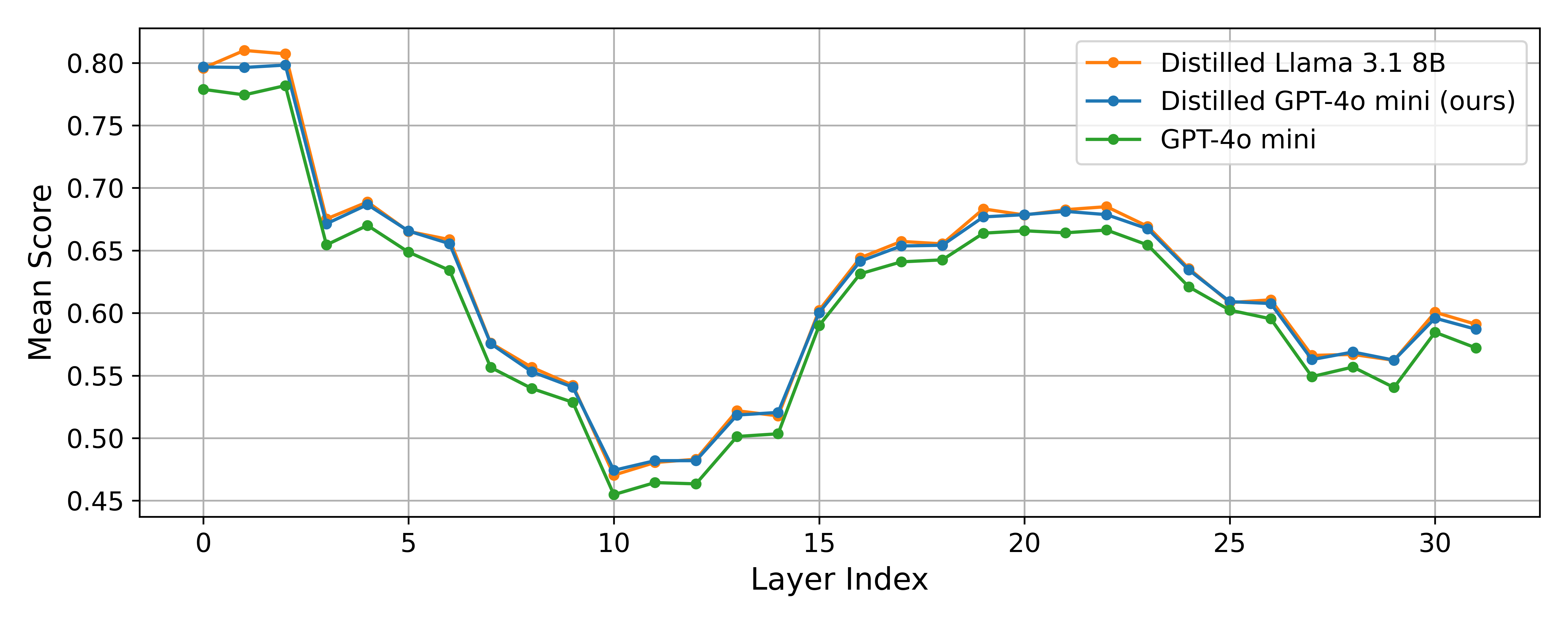
Figure 9: The average-score-per-layer trend is similar for non-finetuned GPT-4o-mini and distilled Llama-3.1-8B-Instruct as distilled GPT-4o-mini. We use 2000 random neurons (the same across all 3 models) to generate this plot (as opposed to all neurons for Figure 1).
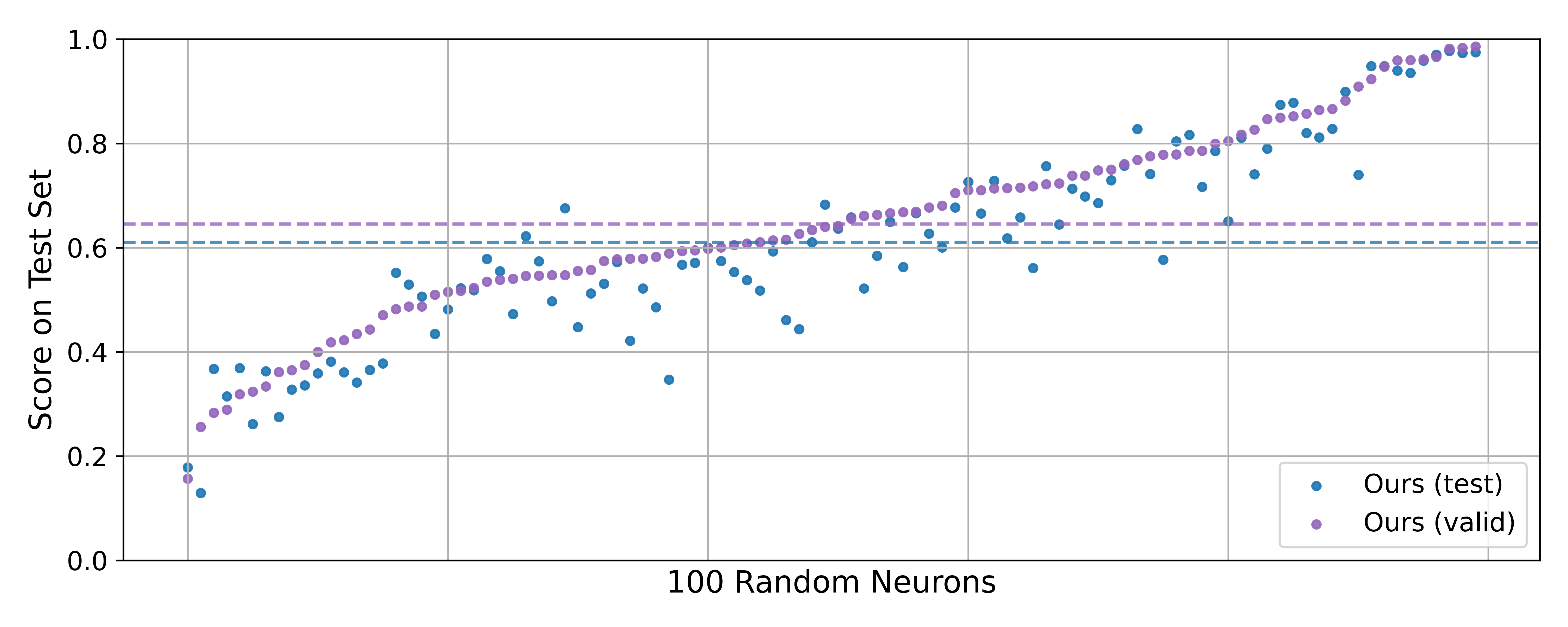
Figure 10: A comparison of simulation scores for our descriptions of 100 random neurons between the validation and test sets of exemplars ( v.s. ). Each description was chosen using best-of-25 sampling over , then evaluated on both and . Although test set scores are often slightly worse than validation set scores, the scores are highly correlated and differ by only 0.04 on average.